Introduction

Poverty in India has been falling consistently since Independence 1The only instance when poverty seemed to have increased is between 2011-12 and 2017-18 based on the leaked report of consumption expenditure for the 2017-18 round. See (Subramanian (2019) for details. . However, progress has not occurred at a constant rate. Poverty reduction during the first decade of the 21st century was particularly rapid. Based on official poverty lines drawn up by the Tendulkar Committee , the headcount rate in India fell from 37 percent of the population in 2004/5 to 22 percent in 2011/12, an annual rate of poverty reduction of more than 2 percentage points per year. A question of considerable interest has been whether this progress has continued or even accelerated in the years since 2011/12.

Establishing how poverty has evolved post-2011/12 is complicated because the micro-data needed to estimate poverty outcomes in a consistent and comparable manner have not been available since the release of the 2011/12 round of the Consumption and Expenditure Survey (CES). In 2017/18, India’s National Sample Survey Organization (NSSO) completed its next quinquennial round of the CES, but these data were not released for public use. Concerns about data quality and reliability were announced, although never clearly and transparently established.

A new round of the CES was completed in 2022/23, but the micro-data from this round have yet to be released. A recently published “Fact Sheet” providing summary tabulations from this survey suggests that poverty in India has fallen dramatically since 2011/12. However, Mehrotra and Kumar (2024), Himanshu (2024), Subramanian (2024), and Ghatak and Kumar (2024) scrutinize this evidence and observe that underlying design changes may affect strict comparability of this most recent CES survey with the 2011/12 round. This suggests that even when the unit record data are released, poverty estimates for 2022/3 may not be directly comparable to those for 2011/12.

In the absence of the preferred CES micro-data with which to compare poverty outcomes over time, a large number of studies and researchers have attempted to estimate how poverty in India has evolved since 2011/12. Leaked tabulated consumption estimates from the 2017/18 CES were scrutinized by Subramanian (2019) who suggested that on the basis of these figures, poverty in India actually rose slightly over this interval. Other researchers have employed a variety of different strategies in their attempts to shed light on the possible evolution of poverty since 2011/12. One prominent line of enquiry has employed survey-to-survey imputation methods in which alternative sources of data are leveraged alongside the 2011/12 CES survey in an effort to substitute for the missing unit-record level CES for 2017/18 and 2022/23.

Much of this imputation-based analysis was undertaken by researchers based at the World Bank, seeking to update the Bank’s estimates of poverty in India so as to be able to feed these into the global poverty estimates that the World Bank publishes on a regular basis 2In fact, all of the poverty estimates used by the World Bank for poverty estimates for India after 2011-12 use this method. . Newhouse and Vyas (2019) model per capita consumption in the 2011/12 CES and impute this consumption into an NSS survey of services and durables collected in 2014/15. Based on the World Bank’s poverty line of $1.90 per person per day in 2011 PPPs, their calculations translate into a decline in poverty in India from 22 percent to just under 15 percent in 2014/15 – a not inconsiderable decline. Edochie et al (2022) undertake a similar imputation exercise but impute consumption from the 2011/12 CES into the NSS’s 2017/18 Survey on Social Consumption of Health. Their estimates indicate that poverty had fallen from 22 percent to just under 10 percent by 2017/18 – suggesting a continuation of the poverty decline reported by Newhouse and Vyas.

Recently, Sinha Roy and van der Weide (2022) investigate poverty trends by scrutinizing consumption data from the private-sector generated Consumer Pyramid Household Survey (CPHS) for 2019 alongside the 2011/12 CES. While the CPHS does collect a measure of consumption, this measure is not directly comparable to that of the CES. Sinha Roy and van der Weide implement a procedure to convert the CPHS consumption measure into one that is more comparable to that of the CES. An additional adjustment is to re-weight the CPHS due to evidence that the CPHS may not be fully representative of the Indian population. Following their adjustments, Sinha Roy and van der Weide estimate poverty in the CPHS and suggest that in 2019 the incidence of poverty in India was slightly over 10 percent (at the $1.90 World Bank poverty line) down from 22.5 per cent in 2011/12. In a robustness check, they also undertake an imputation exercise, where consumption in the 2011/12 CES is predicted into the CPHS on the basis of a set of household characteristics included in both the CES and CPHS. This exercise yields largely similar findings of a decline in poverty of roughly 12 percentage points between 2011/12 and 2019. The calculations by Roy and van der Weide (2022) were formally adopted by the World Bank and have been incorporated into the World Bank’s Poverty and Inequality Platform (PIP). They feed into the World Bank’s global poverty estimates.

As described above, the prevailing estimates from survey-to-survey imputation methods suggest that poverty has fallen markedly since 2011/12. This is in contrast with the findings of Subramanian (2019). Other approaches, employing alternative methods and data, provide a wide range of additional estimates. At one extreme, estimates reported by Bhalla et al (2022) suggest that poverty had been virtually eliminated by 2020. In contrast Ghatak and Kumar (2023) express strong doubts regarding this optimistic view – pointing to sluggish aggregate growth and varying state-level growth rates, the stagnant share of agriculture in total output, and the unchanging share of precarious workers in the labor force. They propose an alternative calculation of poverty in 2019 based on scrutiny of India’s Periodic Labor Force Surveys (PLFS) as well as tabulations from the leaked report from the 2017/18 CES survey. Based on their calculations poverty in India remained at 20-22 percent in 2019/20 – indicating little, if any, poverty decline since 2011/12.

The present study seeks to engage in this debate by proposing yet another imputation-based analysis. Similar to Ghatak and Kumar (2023) we draw on India’s employment surveys for our study. In 2011/12 the NSSO fielded its regular Employment and Unemployment Survey (EUS). This is a companion survey to the 2011/12 CES, based on a very similar sampling design and survey implementation procedures. However, while the EUS does include a consumption module, its somewhat abbreviated consumption aggregate is not directly comparable to the comprehensive consumption measure available in the CES. In 2017/18 the NSSO introduced a new employment survey to replace the EUS. This Periodic Labor Force Survey (PLFS) is modelled very closely on the EUS, but includes only a minimal consumption aggregate that cannot be compared with that in the EUS (or CES) 3These are further complicated due to the change in the questionnaire for collecting consumption aggregates which was based on a single question for 2017-18 and 2018-19 but was expanded to five questions from 2019-20 onwards. . The PLFS is collected yearly, with data available each year from 2017/18 to 2022/23. An attraction of the EUS and PLFS surveys is that, like the CES, they are designed, fielded and administered by the NSSO, follow very similar definitions and procedures, and collect similarly large samples, representative at the state-level.

The strategy followed in this paper involves two steps. First, we compare the consumption aggregates available in the CES and EUS surveys for 2011/12. We establish that the two surveys represent the same underlying Indian population, and that they differ essentially only in that their respective consumption aggregates are not the same. Accordingly, we redefine the Tendulkar poverty lines so that we can replicate in the EUS survey, using the EUS consumption aggregate, the same poverty outcomes as observed in the CES survey at the state and urban/rural sector level. In our second step we implement the survey-to-survey imputation procedure to predict the EUS consumption aggregate into the PLFS surveys from 2017/18 through 2022/23. Applying our re-defined poverty lines to this imputed consumption aggregate in each of the PLFS surveys, we can estimate poverty in the respective PLFS survey years.

Several features of the procedure we implement help, in our view, to strengthen the plausibility of our poverty estimates. First, by undertaking the imputations from the EUS to the PLFS surveys, we are able to add to our imputation models a range of wage and employment variables as predictors of consumption. This is appealing as there exists a large literature linking poverty in India to agricultural wage rates and employment in casual wage labor 4See for example, Acharya, 1989, Deaton and Dreze, 2002, Eswaran, Kotwal, Ramaswami and Wadhwa, 2009, Kijima and Lanjouw, 2003, Lanjouw and Murgai, 2009. . Such labour market variables are also sensitive to broader macro-economic conditions and public transfers, and can be thus expected to reflect changes in such broader conditions. Second, in our study we estimate our imputation models at the state level, and separately for urban and rural areas. This is appealing because it allows for the possibility that “returns” to characteristics such as education, occupation, employment, caste, religion, etc., differ across states and sector. In a country as vast and varied as India, imposing the assumption that parameter estimates are constant over space is restrictive. By estimating poverty at the state and sector level we are also able to produce national-level poverty estimates that are explicitly built up from state and sector level estimates 5This, in fact has been the suggested practice for obtaining national poverty estimates in all the expert groups of the planning commission to estimate poverty. . This offers us an additional window on the plausibility of our national estimates – they must line up with what we understand and believe applies at the subnational level. None of the currently circulating all-India estimates of poverty trends post-2011/12 can be similarly reconciled with state-level trends.

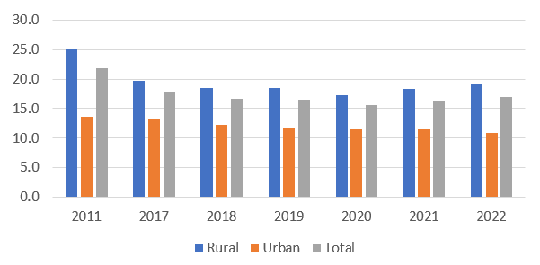
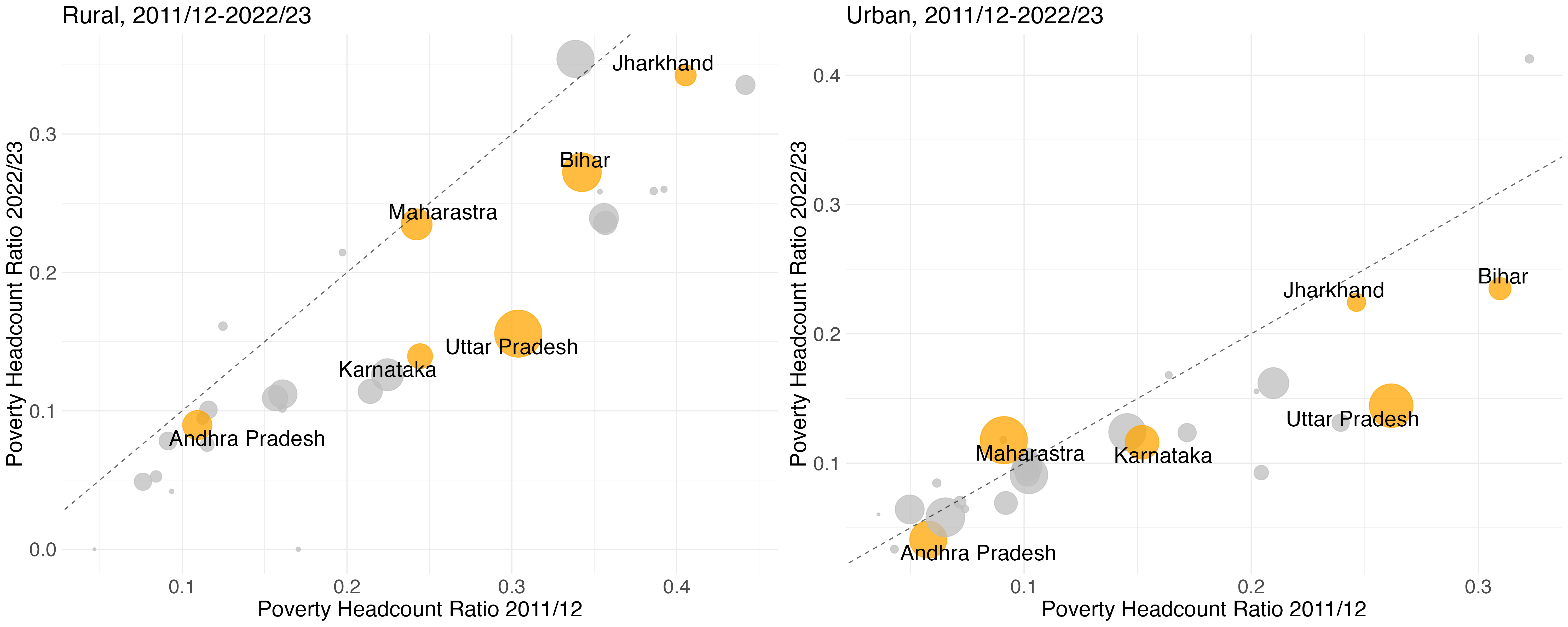
Our estimates suggest that poverty declined only slowly from 2011/12 to 2017/18 and on to 2022/23. From an original estimate of 22 percent of the population in 2011/12 we estimate the incidence of poverty to have fallen to 18 percent by 2017/18 and then further to 17 percent by 2022/23. In rural areas poverty fell from 25 percent to 19 percent between 2011/12 and 2022/23 while in urban areas poverty fell from 14 to 11 percent. This aggregate picture masks considerable variation across states. For example, in Uttar Pradesh poverty is estimated to have nearly halved, from 30 percent in 2011/12 to just over 15 percent in 2022/23. However, in Jharkhand poverty is estimated to have only fallen from 37 to 32 percent between 2011/12 and 2022/23. Similarly, in Bihar poverty is estimated to have only fallen from 34 percent to 27 percent during this interval. It is our contention that credible all-India estimates of how poverty evolved post-2011/12 should resonate with trends at the state level. The question posed by our findings is thus whether these state-level trends make sense and can be corroborated with alternative state-level indicators.

In what follows, we attempt to provide the analytical underpinnings of our estimates in brief. We describe in the next section the general idea behind our imputation method and then follow on from this with a description of the specific implementation strategy employed. In section 4 we turn to a discussion of our results and consider additional corroborating evidence. Section 5 concludes.

Survey-to-Survey Imputation

Survey-to-survey imputation methods for the purpose of poverty measurement are well-established in the literature 6See Dang, et al (2019) and Dang and Lanjouw (2023) for a review of the literature. . Estimating household consumption on the basis of these techniques was initially introduced as part of a small-area estimation approach to poverty measurement (’poverty mapping’) by Elbers et al. (2003) 7See (Elbers et al., 2002), for the working paper version with more details. The idea has been further scrutinized by, for example, Tarozzi and Deaton (2009). . The main idea can be briefly summarized. First, one estimates the relationship between a variable of interest, y (in our case per-capita consumption), and a set of covariates X in a ‘training’ dataset (e.g. the household survey for 2011/12). Next, the model is applied to a second ‘target’ dataset (a survey for 2017/18, say) that includes the same X covariates, but not y. X could include, for example, the education levels of household members, household size, wages earned, etc. By restricting attention to only X variables that are defined in a comparable manner between the two datasets, y can be imputed or ‘predicted’ for all observations in the target dataset 8The underlying assumption here is basically unconfoundedness or ignorability. It requires that y’s distribution conditional on X is the same in both the training and the target datasets. . These imputed values can then generate estimates of poverty at the level one is interested in, e.g. for a whole country or at the state-level.

In choosing which covariates to include in the model, first a list of eligible candidate variables is identified. In our application we employ the Least Absolute Shrinkage and Selection Operator (LASSO) to select the from this list the covariates, X, that can best ‘explain’ the dependent variable, y.

As the imputed value hinges on the variables employed, their choice is crucial. A key assumption of the imputation approach is that the explanatory variables’ effect on the consumption measure should be stable over time. That is, changes in the consumption aggregate between the training and target data thus occur only if the covariates change. If one wishes to credibly track poverty over time (i.e. the training dataset and target dataset represent different time periods) it is thus crucial to not include only stationary or sluggishly moving variables as covariates. Rather, a successful imputation application will include covariates that are both good predictors of consumption expenditure, and that can be expected to change in the face of underlying changing conditions between the training and target datasets. Covariates that might be expected to be useful in the Indian context include detailed wage variables for different income sources or employment characteristics.

The survey-to-survey-methods described above have been implemented in many different studies and contexts 9Early validation studies were reported in Christiaensen et al (2012), Mathiasen (2013), Newhouse et al (2014). Newhouse and Vyas (2019) undertake additional validation analysis based on CES data for 2004/5, 2009/10 and 2011/12. . Dang and Lanjouw (2018) carry out a validation exercise for Indian CES data from 2004/5 into 2009/10. During this interval, India-wide poverty headcounts as captured directly from the 2004/5 and 2009/10 CES surveys, fell from 37.7 percent to 29.9 percent. Dang and Lanjouw (2018) were able to replicate this finding on the basis of imputation models estimated in the 2004/5 survey and applied to the 2009/10 survey. They were thus able to show that the method could capture well even large changes in poverty on the basis of an assumption that ‘returns’ to explanatory variables were constant. As noted above, recent studies by Newhouse and Vyas (2019), Edochie et al (2022) and Sinha Roy and van der Weide (2022) have scrutinized poverty trends since 2011/12 on the basis of these methods as well.

We turn now to a description of the specific application of imputation in the present study.

Poverty in India Post-2011/12

As a discussion of any nuanced concept – particularly within social studies - depends on reliable and stable measures, poverty estimation should be based upon similarly reliable data. For this reason, we choose to impute consumption within - and only within - the surveys that are available from the NSSO. This offers some assurance that we employ consistent underlying concepts for questions, variable definitions, questionnaire design as well as similar sampling and stratification strategies 10Although several socio-economic surveys are available from the NSSO, we prefer to use the surveys which are close to the 2011-12 CES/EUS in sampling, concepts and methodology of data collection. . We also choose the surveys which allow us to have comparable covariates over a time which are good predictors of the variable of interest, consumption expenditure in this case. We also focus on NSS data that employ large samples – able to support estimates at the sub-national, i.e. state, level.

Specifically, we impute from the Employment Unemployment Survey (EUS in 2011/12) into different rounds of the Periodic Labour Force Survey (PLFS 2017/18-2022/23). In contrast to the CES, the EUS data include several appealing labour market and wage indicators. An additional attraction is that the EUS is quite comparable to the PLFS as it was basically its precursor.

We are confronted, however, with the fact that the canonical consumption measure underpinning the official Indian poverty numbers is available only in the CES surveys. Up to 2011/12, all official poverty numbers for India have come out of the comparison of a household’s per capita consumption measure based on this consumption measure with the corresponding poverty line. In other words: we would, ideally, want to continue with this measure as we track poverty beyond 2011/12.

Unfortunately, the CES includes only relatively few household characteristics that are likely to reflect well broader changes in economic circumstance and conditions over time. Sinha Roy and Van Der Weide (2022) point to this limitation as a reason for not basing their preferred estimates on the imputation of consumption from the CES into the PLFS surveys.

The EUS as well as the PLFS surveys, on the other hand, include standard demographic variables as well as an array of labour market and wage variables. As noted earlier, the PLFS, while it is modelled closely on the EUS, does not collect the same consumption aggregate as does the EUS. The EUS consumption aggregate, however, while not identical, is defined and measured in a reasonably similar way to that available in the CES. Both the CES and EUS were surveyed from the same sampling frame in the same time period (July 2011 up to June 2012). This can be seen when comparing overlapping variables between these two surveys. This implies that, the CES and EUS are broadly comparable and represent the same underlying population in 2011/12.

In poverty measurement, the choice of poverty lines is a crucial one. In particular, official poverty estimates for 2011/12 involved comparing consumption in the CES 2011/12 against the poverty lines of the Tendulkar committee. Since the EUS measure of consumption is an abridged version of the measure provided by the CES, a rescaling of the poverty lines applicable to the CES, in order to match the EUS consumption definition, becomes necessary 11This is not a new approach and is identical to the approach used by the Tendulkar committee to arrive at MRP equivalent poverty line for comparison with the earlier URP poverty lines used by the Planning Commission. . For this, we first compute state- and sector-specific poverty rates in the CES. As the EUS represents the same population, we simply have to compute the state and sector-specific poverty lines (in EUS terms) that generate the same poverty rates in the EUS as are produced in the CES with the Tendulkar committee lines 12The underlying assumption behind this procedure is that the estimate of poverty in any year by state/sector is the same irrespective of the distribution and poverty line used. Therefore, for two surveys using different distributions, the poverty lines should be suitably adjusted to yield the same poverty estimate by state/sector. . These are then our rescaled poverty lines. These rescaled poverty lines do not differ too dramatically from the CES ones, but are typically somewhat lower. This is expected, given that EUS consumption is somewhat abbreviated compared to the CES definition. We rely on these ‘rescaled’ poverty lines when imputing consumption from the EUS into the different rounds of PLFS.

It is of interest to examine the overall shape of the consumption distributions based on the CES and EUS surveys, respectively. Figure 1 depicts a zoomed-in comparison of the CES and EUS per capita consumption expenditure distributions. It can be seen that the two distributions are very similarly shaped. This supports the notion that while the EUS consumption definition is somewhat abbreviated relative to that in the CES, its distribution across the population is broadly the same. Table 1 reports the first three moments for each distribution. As expected, the mean in the CES, as well as its standard deviation are slightly higher than in the EUS, but the skewness is quite comparable.

Figure 1: Trimmed density of the consumption measure surveyed in the EUS and CES for the rural and urban population

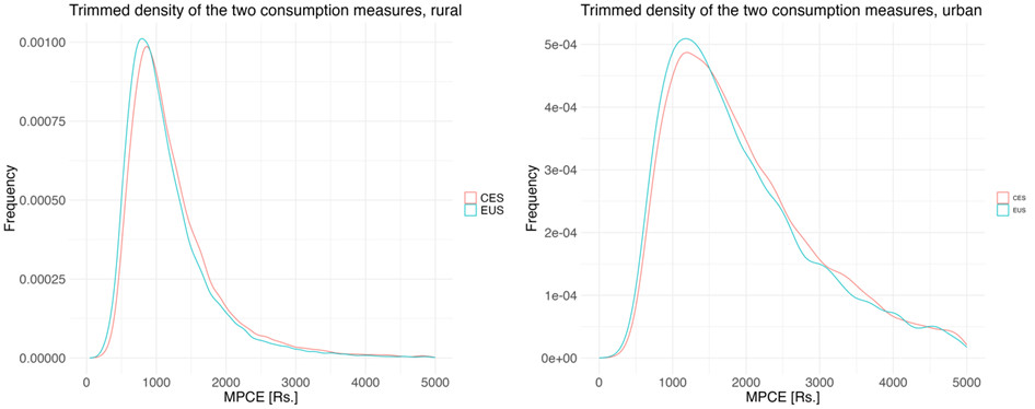
Table 1: Comparison of the first three moments of the CES and EUS consumption measures’ distributions

Another check for equivalence of the distributions is to look at additional poverty measures in the EUS, on the basis of our rescaled Tendulkar committee CES poverty lines (see Table 2). As expected, the poverty headcount ratios lie quite closely to each other. But also, the poverty gap and the squared poverty gap indices are clearly aligned.

Table 2: Comparison of the arising poverty measurements when using the Tendulkar committee poverty lines for the CES dataset and rescaled poverty lines for the EUS

Further details of the comparison of the CES with the EUS can be found in (Himanshu, Lanjouw and Schirmer, 2024).

India’s heterogeneity across states and regions is widely acknowledged. Poverty outcomes correspondingly vary sharply across states and urban/rural sectors 13See Drèze and Srinivasan (1996), Deaton and Drèze (2002), Kijima and Lanjouw (2003), and World Bank (2008). . It is thus somewhat surprising to see that earlier imputation-based approaches to gauging the evolution of poverty since 2011/12 rely on a single, nation-wide, model for rural and urban areas respectively. We suggest that state-level models are more appealing. With these, differences between states can be captured in both selection of variables as well as their respective effect on consumption. Accordingly, we estimate a separate urban and rural model in each state. This also allows us to estimate and report state-level poverty rates.

In allowing for state-sector-specific models, the choice of variable selection becomes even more crucial. In our preferred approach, we pre-define a list of demographic and household characteristics, as well as clearly changing labour market and wage variables. We then use LASSO to produce a first pass at a state-sector specific model. This generally provides us with high explanatory power of the model, measured in Adj. R². However, these models have two issues we address in a second step. First, although LASSO generally yields good overall explanatory power, it can lead to the inclusion of individually insignificant regressors. Second, LASSO does not necessarily guarantee selection into the model of labour market variables. Thus, we impose inclusion of those wage and labour market variables that were disregarded by LASSO. We then, eliminate, one by one, those non-labour variables that have a p-value of more than 0.05. In this way, we can arrive at fairly parsimonious models with acceptable explanatory power that are assured of also including some of the labour market variables we feel are important for capturing changes in broad economic conditions.

Equipped with these models, we can then impute consumption into the different rounds of the PLFS. Since we want to gauge poverty changes at both the national and state-level, the final estimates are reported at these two levels.

Results

Based on our preferred models, we compute poverty headcount ratios for the whole country from 2011/12 up to 2022/23. As can be seen in Figure 2, poverty in India as a whole fell modestly between 2011/12 and 2017/18. In the subsequent years, leading up to COVID, we see a further, slight, fall in poverty. With the Covid-19 outbreak, a reversal in this trend takes place. This is clearly visible for the two-thirds of the population that reside in rural areas. For the urban population, it is less clearly discernable.

Figure 2: Poverty headcount ratio for the rural, urban and total population (2011- 2023)

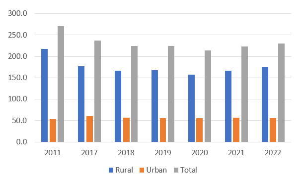
As India grew, not only economically, but also in terms of population, it is of interest to ask how the absolute number of poor people evolved over time. The Indian population grew by about 200 million people between the 2011/12 EUS and the last round of the PLFS survey. The numbers of poor follow a similar trajectory as was observed for the poverty ratio. Strikingly, Figure 3 shows that in 2022/23 the number of poor people in India had not fallen beyond the number in 2018.

Figure 3: Number of Poor in India (in Millions, Tendulkar committee poverty lines)

Unlike the other estimates in circulation, our all-India poverty estimates are built up from state and sector-level estimates. This offers a reality check on the all-India estimates, by allowing one to scrutinize levels and trends of poverty at the state-level. Figures 4a and 4b highlight state-level trends for a selection of states. In Figure 4a respective rural and urban poverty rates in all states are depicted for 2017/18. Note that all states uniformly show either no, or declining poverty, since 2011/12. Generally, those states that were poorer in 2011/12 experienced larger declines in poverty. This accords with the general notion of poverty convergence. Figure 4b compares poverty between 2011/12 and 2022/23. Substantial poverty decline is evident in both rural and urban Uttar Pradesh. Other historically poor states, notably Jharkhand and Bihar, point to much slower progress.

Figure 4a: State-level poverty headcount ratios of the rural and urban population

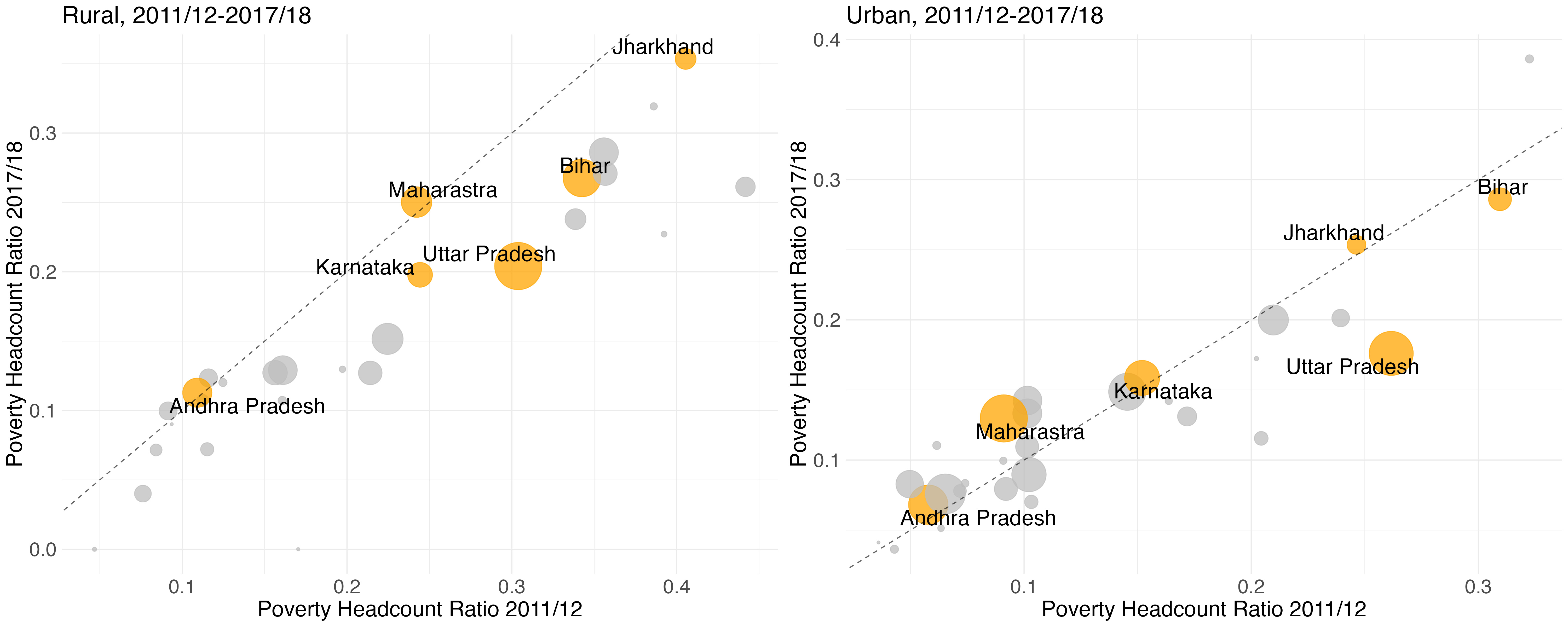
Figure 4b: State-level poverty headcount ratios of the rural and urban population

Concluding Discussion

The results presented in this article point to a more modest decline in poverty using the survey-to-survey imputation methodology than estimates available from the World Bank using similar methods. Part of the difference between our estimates and the other estimates is the choice of survey datasets. We have used the NSSO surveys which are conceptually and practically similar to the CES and the EUS, and which allow us to use a larger set of variables that are strong proxies of the consumption in the CES. In particular, by employing the EUS and PLFS surveys we have been able to include wages and earnings along with employment characteristics as predictors of poverty. These predictors are not available in the various World Bank estimates that are based on alternative datasets. A further, significant, reason for our estimates differing from those of the World Bank is due to our application of survey-to-survey imputation methods at the state level, and separately for rural and urban areas. Our all-India estimates of poverty are thus built up from state-level estimates, rather than treating rural/urban India as a single unit.

While our estimates suggest a modest decline in poverty compared to World Bank estimates, they are similar to other estimates such as those reported by Ghatak and Kumar (2023). In that study, all-India poverty is estimated at 19.6 percent in 2017-18 and 16.8 percent in 2018-19. This is not far from our findings of 17.8 percent in 2017-18 and 16.6 percent in 2018-19. Although their regression-based estimates are higher than ours for 2017-18, both studies suggest a decline in 2018-19 compared to 2017-18. Our estimates are also close to the estimates reported by the India Employment Report (2024) which estimates poverty at 18.2 percent in rural India and 12.5 percent in urban India in 2022-23 14See India Employment Report (2024), prepared by International Labour Organisation and Institute for Human Development. The report uses the consumption aggregates from the PLFS surveys adjusted to establish comparability with the CES consumption surveys. . Our estimates for 2022-23 are marginally higher at 19.2 percent in rural India but lower at 10.8 percent in urban India.

Our estimates are also consistent with indicators of wages and earnings from internally consistent NSSO surveys but also a wide variety of external data on wages, earnings and employment characteristics. At the aggregate level, most indicators of national income as well as earnings of workers suggests a declining growth rate of real incomes. Table 3 presents some broad indicators of income and earnings for different class of workers. While casual wages from the NSSO show slowing growth during 2011-12 to 2022-23 compared to the 2004-05 to 2011-12 period, the deceleration is sharper in case of rural workers. In contrast to rural areas, regular workers have seen an actual decline in real earnings from regular employment during the later period, compared to the growth during 2004-05 and 2011-12. Even real incomes of cultivators show a sharp deceleration using the disaggregated data from the national accounts.

Table 3: Some broad indicators of income and earnings

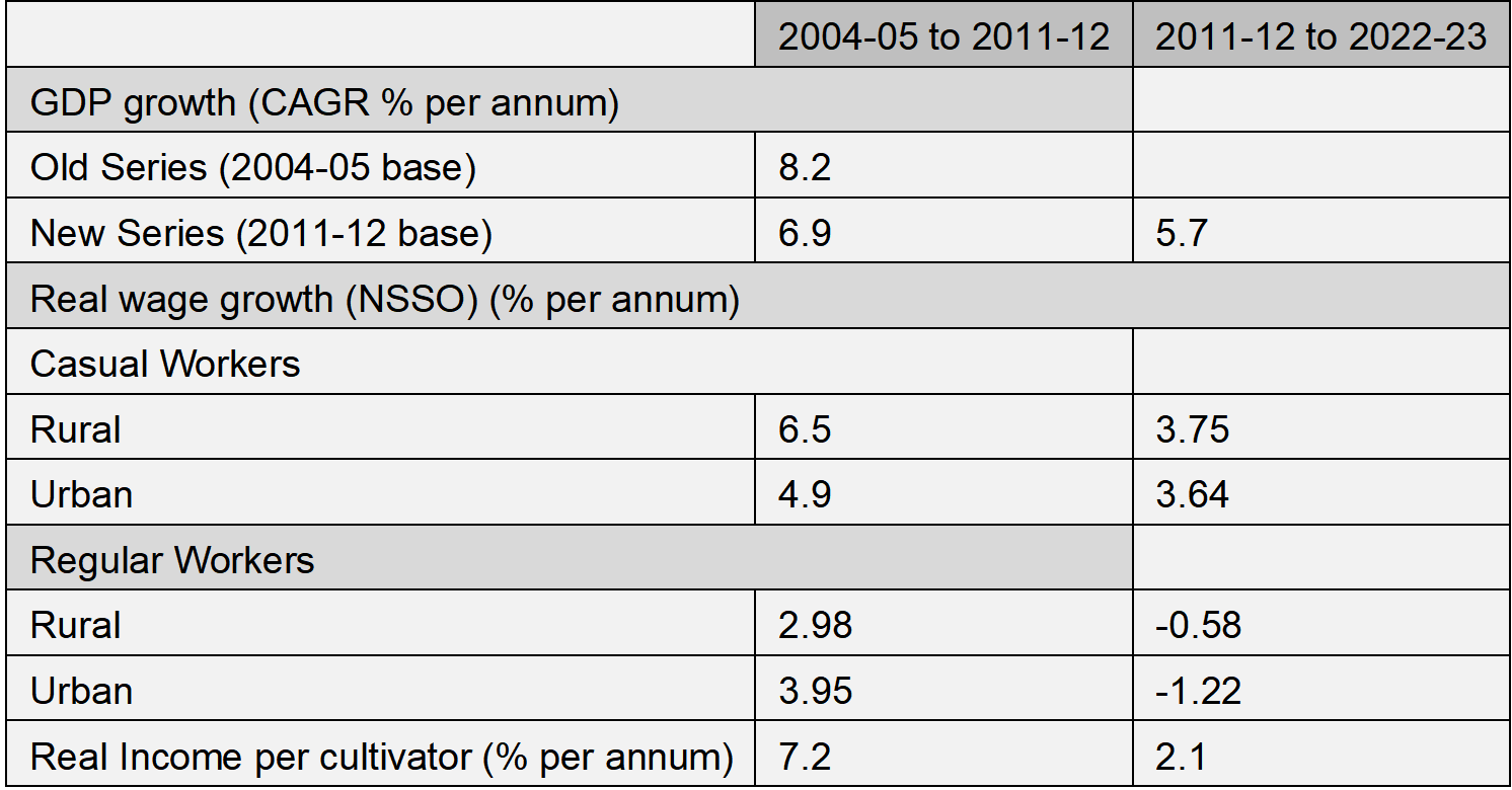
Note: Real Income per cultivator is based on the methodology suggested by the NITI Aayog Policy Paper (2017). 15See Chand (2017) for details

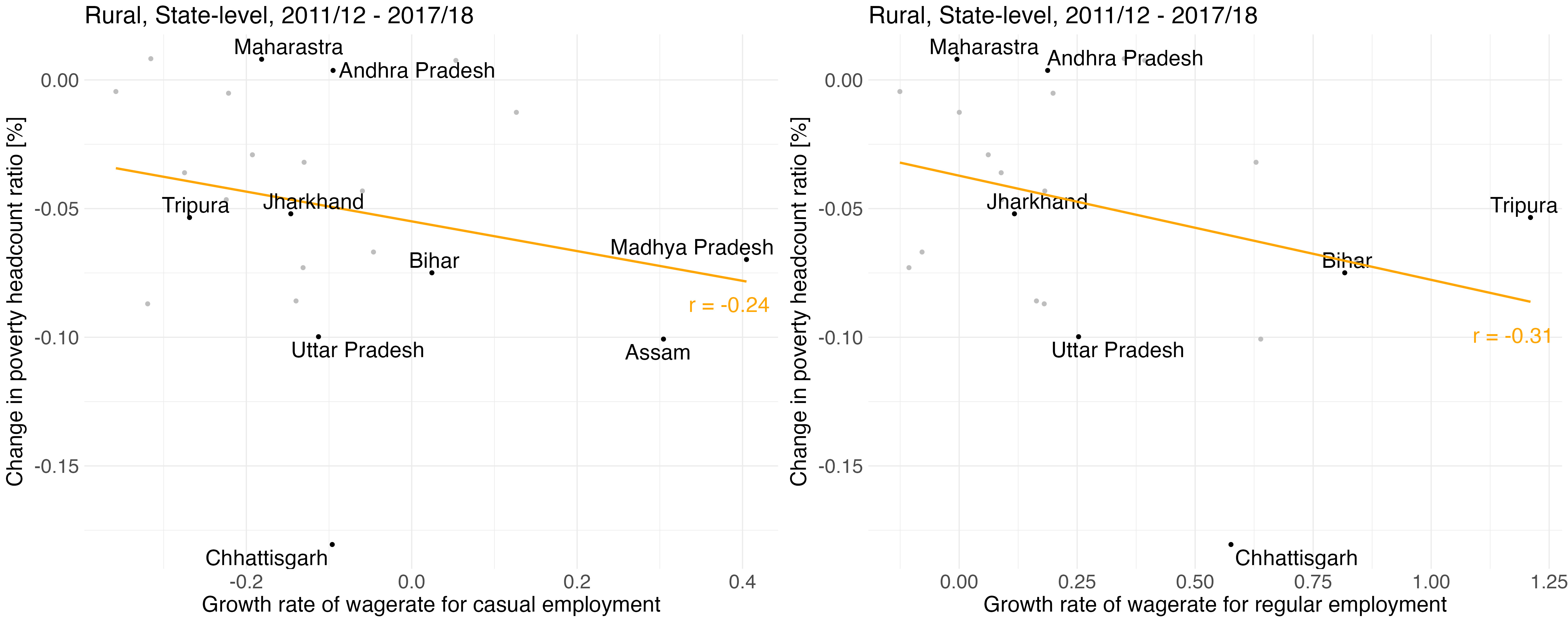
Our estimates also correlate with data on incomes and earnings at the state level. Figure 5 illustrates this for rural areas by plotting changes in state-level poverty headcounts against growth in casual wages and earnings from regular, salaried, employment, respectively. While considerable variation across states can be observed, there is a clear pattern of more substantial poverty reduction in states that saw more rapid increases in employment earnings.

Figure 5: Changes in state-level rural poverty headcount ratios against growth in earnings from casual, and regular, wage employment

As noted earlier, NSSO recently released a fact sheet on the preliminary results from the 2022-23 survey of consumer expenditure. Unfortunately, the 2022-23 survey was conducted with a completely new questionnaire, multiple visit surveys and a different sampling design. While these modifications may be useful for the purpose of GDP revision and Price Index revision, the 2022-23 consumption data cannot be directly scrutinized for the purpose of poverty analysis given the differences in the methodology of data collection. The present study has tried to fill the gap on the vexed question of what happened to poverty after 2011-12 by employing widely-employed survey-to-survey imputation methods. While, inevitably, caveats remain even in our case, notably regarding the assumption on stability of regression coefficients over time, there are grounds for believing that this survey-to-survey based analysis offers us a reasonable picture of changes in poverty over time. The methodology is appealing as it is less vulnerable to changes in underlying data collection methods. It is also well suited to the present situation where poverty lines have not yet been defined for the 2022-23 consumption expenditure definition. While the estimates presented in this article are consistent with other indicators and studies pointing to a slower decline in poverty after 2011-12, a definitive assessment of changes in poverty will ultimately require that the NSSO conducts a bridge survey comparable to the 2011-12 consumption survey. Until then, the debate is unlikely to be fully resolved.

Himanshu is with Jawahrlal Nehru University. Peter Lanjouw is with Vrije Universiteit Amsterdam, Netherlands, and Tinbergen Institute, Amsterdam, Netherlands. Philipp D. Schirmer is with Vrije Universiteit Amsterdam, Netherlands and Tinbergen Institute, Amsterdam, Netherlands.

This article is based on a more extensive analysis reported in Himanshu, Lanjouw and Schirmer (2024). The project is part of the Oxford Policy Management DEEP project undertaken on behalf of the Foreign Commonwealth and Development Office of the UK. We are grateful for useful discussions with Chris Elbers, Maitreesh Ghatak, Rishabh Kumar, Roy van der Weide, and participants at the 2024 Winter School on Inequality and Social Welfare Theory, Canazei, Italy.

This is the third article in this symposium on poverty estimates in India. The first two article were published on April 5 and April 12.